This page is designed to explain how ?lpdf objects can
be used for automated learning of hyperparameters and general fitting of
predictors.
Let’s set things up for a 3 dimensional example.
om = new(outermod)
d = 3
setcovfs(om, rep("mat25pow",d))
knotlist = list(seq(0.01,0.99,by=0.02),
                seq(0.01,0.99,by=0.02),
                seq(0.01,0.99,by=0.02))
setknot(om, knotlist)
Hyperparameter impact
The values of covariance function hyperparameters are extremely
important for successful near-interpolation of surfaces. This impact is
felt in outerbase and this section is designed to
illustrate that.
Consider the first four basis functions plotted below.
sampsize = 30
design1d = seq(1/(2*sampsize),1-1/(2*sampsize),1/sampsize)
x = cbind(design1d,sample(design1d),sample(design1d))
ob = new(outerbase, om, x)
basis_func0 = ob$getbase(1)
matplot(x[,1],basis_func0[,1:4],
        type='l', ylab="func", xlab="first dim")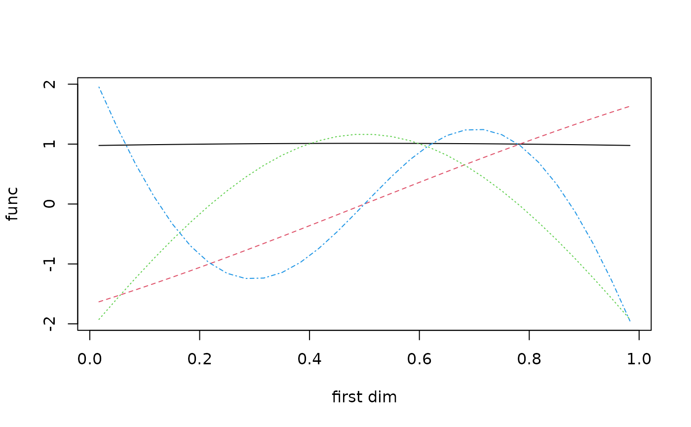
The hyperparameters will now be changed in a way that we know will
change these basis functions. Note that ob$build is
required after updating the hyperparameters for it to take effect as
ob does not know when om is updated.
hyp0 = gethyp(om)
hyp0[2] = 3 #changing the power on first parameter
om$updatehyp(hyp0)
ob$build() #rebuild after updatehyp
This leads to an asymmetric basis function set for this first
dimension because of the power transform in
?covf_mat25pow.
basis_func1 = ob$getbase(1)
matplot(x[,1],basis_func0[,1:4],
        type='l', ylab="func", xlab="first dim",
        main="original hyperparameters")
matplot(x[,1],basis_func1[,1:4],
        type='l', ylab="func", xlab="first dim",
        main="new hyperparameters")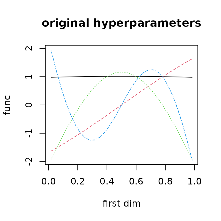

lpdf for learning
The core building block for outerbase learning is the base class
?lpdf, log probability density functions. This base class
forms the backbone behind learning using statistical models. Instances
of this class allow us to optimize coefficients, infer on uncertainty
and learn hyperparameters of covariance functions.
A small dataset can illustrate (almost) all core concepts related to
lpdf.
y = obtest_borehole3d(x)The length of the hyperparameters is 2 dimensions for each covariance function for a total of 6 hyperparameters.
gethyp(om)
#> inpt1.scale inpt1.power inpt2.scale inpt2.power inpt3.scale inpt3.power
#>           0           3           0           0           0           0
hyp0 = c(-0.5,0,-0.5,0,-0.5,0)
om$updatehyp(hyp0)
We will use 60 terms to build our approximation.
terms = om$selectterms(60)The idea is to build a loglik object that represent that
log likelihood of our data given the model and coefficients. We will
begin with ?loglik_std, although this model is not
recommended for speed reasons. We can initialize it and check that we
can get gradients with respect to coefficients, covariance
hyperparameters, and parameters of the lpdf object
itself.
loglik = new(loglik_std, om, terms, y, x)
coeff0 = rep(0,loglik$nterms)
loglik$update(coeff0) # update it to get gradients
loglik$val
#> [1] -176.6428
head(loglik$grad) # dim 60 for number of coeffients
#>            [,1]
#> [1,] -0.4059074
#> [2,] -0.7181826
#> [3,]  1.1517755
#> [4,]  4.5333041
#> [5,] -0.2309182
#> [6,] -0.3139779
A reasonable statistical model also needs prior on the coefficients. This tells us what distribution we expect on the coefficients.
logpr = new(logpr_gauss, om, terms)To make the handling of these two objects loglik and
logpr easier, the ?lpdfvec class is helpful to
tie the objects together. It will share the hyperparameter vector
between them, so they need to be based on the same outermod
object. But it will concatenate the parameters.
logpdf = new(lpdfvec, loglik, logpr)
para0 = getpara(logpdf)
para0
#> noisescale coeffscale
#>   2.730834   6.000000
para0[2] = 4
logpdf$updatepara(para0)
getpara(logpdf)
#> noisescale coeffscale
#>   2.730834   4.000000
The coefficients coeff are considered ancillary
parameters that need to be optimized out (or something more
sophisticated, hint on current research). For this class, it is easiest
to do this via lpdf$optnewton, which takes a single Newton
step to optimize the coefficients.
logpdf$optnewton()Some test data will help illustrate prediction.
testsampsize = 1000
xtest = matrix(runif(testsampsize*d),ncol=d)
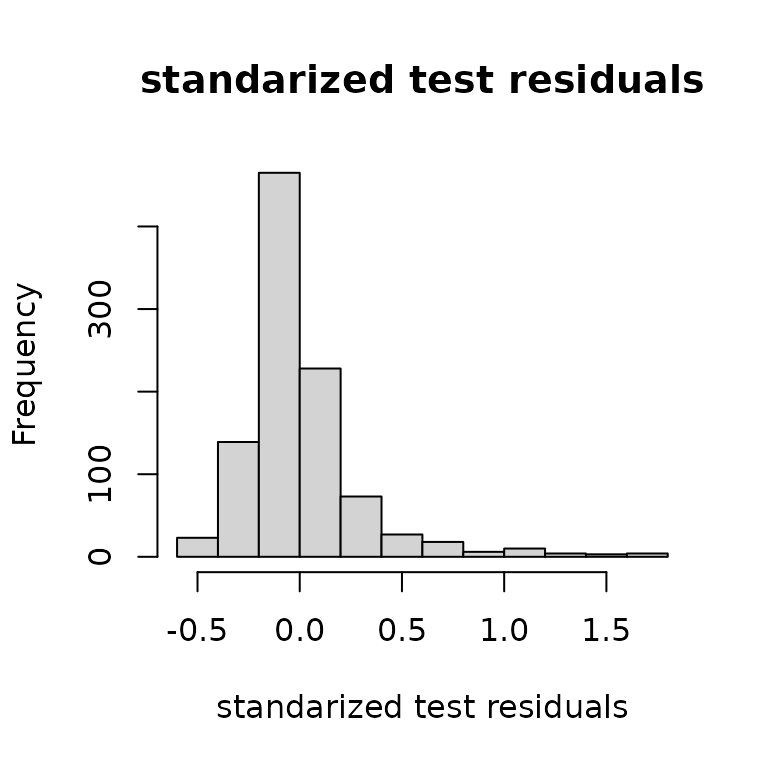
ytest = obtest_borehole3d(xtest)We can see the predictive accuracy using the ?predictor
class which automatically pulls correct information out of
loglik to design predictions.
predt = new(predictor,loglik)
predt$update(xtest)
yhat = as.vector(predt$mean())
varpred = as.vector(predt$var())

plot(yhat,ytest, xlab="prediction", ylab="actual")
hist((ytest-yhat)/sqrt(varpred),
     main="standarized test residuals",
     xlab = "standarized test residuals")
lpdf and hyperparameters
The main value in this approach is the automated pulling of important gradients related to covariance hyperparameters and model parameters.
logpdf$optnewton()
logpdf$gradhyp    # dim 6 for all hyperparameter
#>            [,1]
#> [1,] -0.8816823
#> [2,]  0.2532020
#> [3,]  9.8633096
#> [4,]  1.0109075
#> [5,] 10.5203974
#> [6,]  1.1226996
logpdf$gradpara   # dim 2 since 2 parameters
#>            [,1]
#> [1,] -16.573513
#> [2,]  -4.127843
This allows us to use custom functions to learn these hyperparameters
to give maximum predictive power. The goal right now is a single point
estimate of these hyperparameters. One has to be very careful to keep
these in good ranges, and the call below will make sure to return
-inf if there is a problem with the chosen
hyperparameters.
totobj = function(parlist) { #my optimization function for tuning
  regpara = logpdf$paralpdf(parlist$para) # get regularization for lpdf
  reghyp = om$hyplpdf(parlist$hyp) # get regularization for om
  if(is.finite(regpara) && is.finite(reghyp)) { # if they pass
    om$updatehyp(parlist$hyp)        # update hyperparameters
    logpdf$updateom()             # update the outerbase inside
    logpdf$updatepara(parlist$para)  # update parameter
    logpdf$optnewton()            # do opt

    gval = parlist #match structure
    gval$hyp = -logpdf$gradhyp-om$hyplpdf_grad(parlist$hyp)
    gval$para = -logpdf$gradpara-logpdf$paralpdf_grad(parlist$para)
    list(val = -logpdf$val-reghyp-regpara, gval = gval)
  } else list(val = Inf, gval = parlist) }
This works by querying the objects themselves to check if the
parameters are reasonable. This package provides a custom deployment of
BFGS in ?BFGS_std to optimize functions like
this.
parlist = list(para = getpara(logpdf), hyp = gethyp(om))
totobj(parlist)
#> $val
#> [1] 80.31398
#>
#> $gval
#> $gval$para
#>           [,1]
#> [1,] 16.573513
#> [2,]  3.627843
#>
#> $gval$hyp
#>            [,1]
#> [1,]  -4.475461
#> [2,]  -0.253202
#> [3,] -15.220452
#> [4,]  -1.010908
#> [5,] -15.877540
#> [6,]  -1.122700
opth = BFGS_std(totobj, parlist, verbose=3) #
#>
#> ########started BFGS#######
#>  iter.no obj.value wolfe.cond.1 wolfe.cond.2 learning.rate
#>        0    80.314           NA           NA           0.1
#>  iter.no obj.value wolfe.cond.1 wolfe.cond.2 learning.rate
#>        1   77.0321      -3.2813     -45.8753           0.1
#>  iter.no obj.value wolfe.cond.1 wolfe.cond.2 learning.rate
#>        2   71.7493     -5.28223    -0.553311       0.50357
#>  iter.no obj.value wolfe.cond.1 wolfe.cond.2 learning.rate
#>        3   57.1662      -14.581     -24.7129      0.539329
#>  iter.no obj.value wolfe.cond.1 wolfe.cond.2 learning.rate
#>        4    53.102     -4.06372      -1.9579      0.573679
#>  iter.no obj.value wolfe.cond.1 wolfe.cond.2 learning.rate
#>        5   44.6069     -8.49404     -5.31126      0.606459
#>  iter.no obj.value wolfe.cond.1 wolfe.cond.2 learning.rate
#>        6   33.9651     -10.6403     -11.0213      0.637561
#>  iter.no obj.value wolfe.cond.1 wolfe.cond.2 learning.rate
#>        7   29.3316     -4.63289     -5.21781      0.666913
#>  iter.no obj.value wolfe.cond.1 wolfe.cond.2 learning.rate
#>        8   27.9386     -1.39271      -3.9757      0.694484
#>  iter.no obj.value wolfe.cond.1 wolfe.cond.2 learning.rate
#>        9   27.4111    -0.527351     -1.87134      0.720271
#> num iter: 10  obj start: 80.31398  obj end: 27.36843
#> final learning rate: 0.7442976
#> approx lower bound (not achieved): 27.28692
#> #########finished BFGS########
Then we just have to update out parameters and re-optimize, and we can check that we are at least must closer to stationary point.
totobj(opth$parlist)
#> $val
#> [1] 27.36843
#>
#> $gval
#> $gval$para
#>            [,1]
#> [1,] -0.5660887
#> [2,] -1.3153120
#>
#> $gval$hyp
#>             [,1]
#> [1,]  0.08840577
#> [2,] -0.01943364
#> [3,] -0.28713673
#> [4,]  0.03055821
#> [5,] -0.08254016
#> [6,]  0.20042590
These steps can all be nicely wrapped up in another function
?BFGS_lpdf, which is a simpler call with the same result.
Note because of some things not fully understood, these numbers will not
match exactly above, but they will be quite close and
functionally the same.
opth = BFGS_lpdf(om, logpdf,
                 parlist=parlist,
                 verbose = 3, newt= TRUE)
#>
#> ########started BFGS#######
#>  iter.no obj.value wolfe.cond.1 wolfe.cond.2 learning.rate
#>        0    80.314           NA           NA           0.1
#>  iter.no obj.value wolfe.cond.1 wolfe.cond.2 learning.rate
#>        1   77.0321      -3.2813     -45.8753           0.1
#>  iter.no obj.value wolfe.cond.1 wolfe.cond.2 learning.rate
#>        2   71.7493     -5.28223    -0.553311       0.50357
#>  iter.no obj.value wolfe.cond.1 wolfe.cond.2 learning.rate
#>        3   57.1662      -14.581     -24.7129      0.539329
#>  iter.no obj.value wolfe.cond.1 wolfe.cond.2 learning.rate
#>        4    53.102     -4.06372      -1.9579      0.573679
#>  iter.no obj.value wolfe.cond.1 wolfe.cond.2 learning.rate
#>        5   44.6069     -8.49404     -5.31126      0.606459
#>  iter.no obj.value wolfe.cond.1 wolfe.cond.2 learning.rate
#>        6   33.9651     -10.6403     -11.0213      0.637561
#>  iter.no obj.value wolfe.cond.1 wolfe.cond.2 learning.rate
#>        7   29.3316     -4.63289     -5.21781      0.666913
#>  iter.no obj.value wolfe.cond.1 wolfe.cond.2 learning.rate
#>        8   27.9386     -1.39271      -3.9757      0.694484
#>  iter.no obj.value wolfe.cond.1 wolfe.cond.2 learning.rate
#>        9   27.4111    -0.527351     -1.87134      0.720271
#> num iter: 10  obj start: 80.31398  obj end: 27.36843
#> final learning rate: 0.7442976
#> approx lower bound (not achieved): 27.28692
#> #########finished BFGS########
The revised predictions are then built after hyperparameter optimization where we find improved predictive accuracy in nearly every category. Here we can see a much better alignment between predictions and actual alongside a better plot of standardized residuals (more like a standard normal distribution).
predtt = new(predictor,loglik)
predtt$update(xtest)
yhat = as.vector(predtt$mean())
varpred = as.vector(predtt$var())

plot(ytest,yhat)
hist((ytest-yhat)/sqrt(varpred), main="standarized test residuals",
     xlab = "standarized test residuals")
