Speeding up inference • outerbase

This page is designed to explain how outerbase can facilitate fast inference with smart modeling choices.

library(outerbase)

The potential benefits grow as the sample size grows. We use a sample size of 500 here in the spirit of running quickly. The point will be obvious, but more dramatic results can be had by increasing the sample size.

sampsize = 500
d = 8
x = matrix(runif(sampsize*d),ncol=d)
y = obtest_borehole8d(x)

First setup an outermod object.

om = new(outermod)
setcovfs(om, rep("mat25pow",8))
knotlist = list();
for(k in 1:d) knotlist[[k]] = seq(0.01,1,by=0.025)
setknot(om, knotlist) #40 knot point for each dim

More data should mean more basis functions. So we will choose 250 terms for our feature space approximation.

p = 250
terms = om$selectterms(p)

Different models

To begin, lets use ?loglik_std to represent our slow approach.

loglik_slow = new(loglik_std, om, terms, y, x) 
logpr_slow = new(logpr_gauss, om, terms)
logpdf_slow = new(lpdfvec, loglik_slow, logpr_slow)

logpdf_slow can be optimized using lpdf$optnewton.

logpdf_slow$optnewton()

Newton’s method involves solving a linear system, thus it takes one step, but is expensive.

?loglik_gauss is a lpdf model designed for speed. It is a nice comparison because loglik_gauss uses the same model as loglik_std, with a few approximations for speed.

loglik_fast = new(loglik_gauss, om, terms, y, x) 
logpr_fast = new(logpr_gauss, om, terms)
logpdf_fast = new(lpdfvec, loglik_fast, logpr_fast)

logpdf_fast will through an error if you try to use optnewton. This is because it is written so that it never builds a Hessian (hess in the code) matrix.

logpdf_fast$optnewton()
#> Error in eval(expr, envir, enclos): addition: incompatible matrix dimensions: 0x0 and 250x250

It is instead suggested to use lpdf$optcg (conjugate gradient) to optimize the coefficients in the fast version.

logpdf_fast$optcg(0.001,  # tolerance
                  100)    # max epochs

As an aside, omp speed ups are possible, but you need to have correctly compiled with omp. One check is to call the following.

ob = new(outerbase, om, x) 
ob$nthreads
#> [1] 2

If the answer is 1 but you have a multicore processor (most modern processors), your installation might be incorrect.

You can manually set the number of threads for lpdf objects.

logpdf_slow$setnthreads(4)
logpdf_fast$setnthreads(4)

Timing

The main cost of fitting outerbase models is hyperparameter optimization. The difference between logpdf_slow and logpdf_fast will be apparent. Let’s save starting points (since they share om) for fairness.

parlist_slow = list(para = getpara(logpdf_slow), hyp = gethyp(om))
parlist_fast = list(para = getpara(logpdf_fast), hyp = gethyp(om))

Test points will verify the predictions are equally good with either model, the only difference is speed.

xtest = matrix(runif(1000*d),ncol=d) #prediction points
ytest =  obtest_borehole8d(xtest)

We will use the unsophisticated proc.time to do some quick timing comparisons.

ptm = proc.time()
opth = BFGS_lpdf(om, logpdf_slow, 
                 parlist=parlist_slow, newt=TRUE)    
t_slow = proc.time() - ptm
pred_slow = new(predictor,loglik_slow)
pred_slow$update(xtest)
yhat_slow = as.vector(pred_slow$mean())
print(t_slow)
#>    user  system elapsed 
#>   7.965   1.900   5.200

ptm = proc.time()
opth = BFGS_lpdf(om, logpdf_fast, 
                 parlist=parlist_fast, newt=FALSE)  
t_fast = proc.time() - ptm
pred_fast = new(predictor,loglik_fast)
pred_fast$update(xtest)
yhat_fast = as.vector(pred_fast$mean())
print(t_fast)
#>    user  system elapsed 
#>   4.449   1.410   3.055

Comparison of results

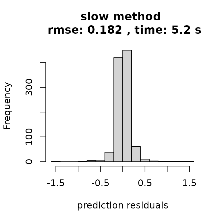
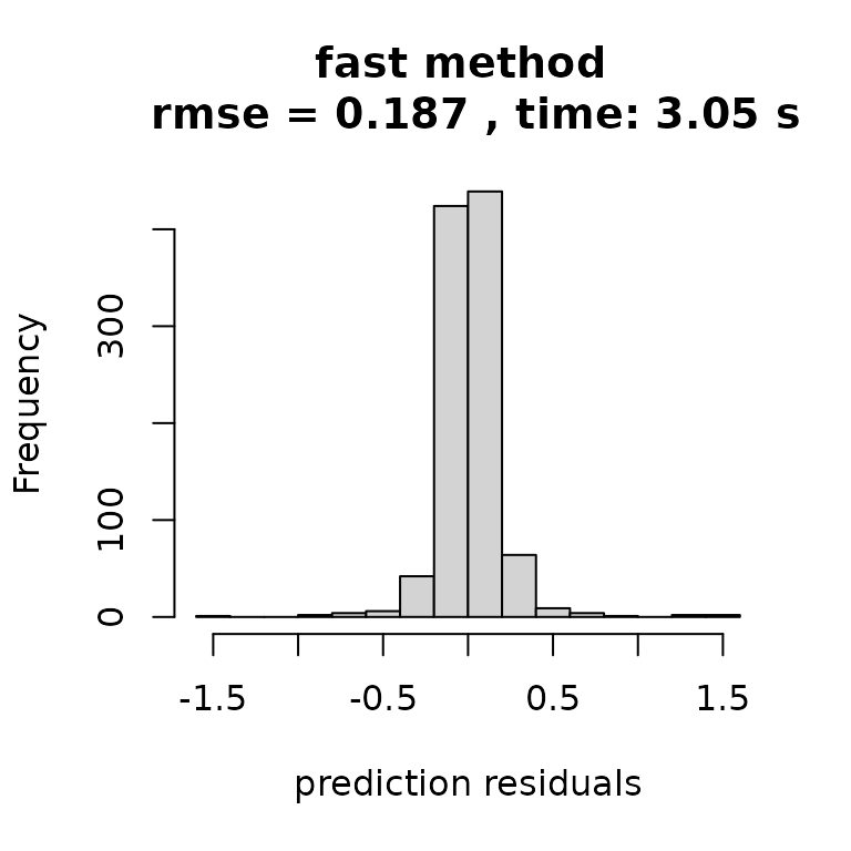
And simply plotting the results tells the story: faster inference with no discernible drop off in quality. Note there are serious approximations here, but the approximations just have a negligible effect.

rmse_slow = sqrt(mean((ytest-yhat_slow)^2))
hist((ytest-yhat_slow), main=paste("slow method \n rmse:", 
                                    round(rmse_slow,3),
                                   ", time:",
                                   round(t_slow[3],2),'s'),
     xlab = "prediction residuals")
rmse_fast = sqrt(mean((ytest-yhat_fast)^2))
hist((ytest-yhat_fast), main=paste("fast method \n rmse =",
                                      round(rmse_fast,3),
                                   ", time:",
                                   round(t_fast[3],2),'s'), 
     xlab = "prediction residuals")